Machine Learning Crash Course: Part 2
24 Dec 2016 | Daniel Geng and Shannon ShihPerceptrons, Logistic Regression, and SVMs
In this post we’ll talk about one of the most fundamental machine learning algorithms: the perceptron algorithm. This algorithm forms the basis for many modern day ML algorithms, most notably neural networks. In addition, we’ll discuss the perceptron algorithm’s cousin, logistic regression. And then we’ll conclude with an introduction to SVMs, or support vector machines, which are perhaps one of the most flexible algorithms used today.
Supervised and Unsupervised Algorithms
In machine learning, there are two general classes of algorithms. You’ll remember that in our last post we discussed regression and classification. These two methods fall under the larger umbrella of supervised learning algorithms, one of two classes of machine learning algorithms. The other class of algorithms is called unsupervised algorithms.
Supervised algorithms learn from labeled training data. The algorithms are “supervised” because we know what the correct answer is. If the algorithm receives a bunch of images labeled as apples or oranges it can first guess the object in the image, then use the label to check if its guess is correct.
Unsupervised learning is a bit different in that it finds patterns in data. It works similarly to the way we humans observe patterns (or objects) in random phenomena. Unsupervised learning algorithms do the same thing by looking at unlabeled data. Just like we don’t have a particular goal when looking at an object (other than identifying it), the algorithm doesn’t have a particular goal other than inferring patterns from the data itself.
We’ll talk about unsupervised algorithms in a later blog post. For now, let’s look at a very simple supervised algorithm, called the perceptron algorithm.
Perceptrons

Model of a perceptron
One of the goals of machine learning and AI is to do what humans do and even surpass them. Thus, it makes sense to try and copy what makes humans so great at what they do–their brains.
The brain is composed of billions of interconnected neurons that are constantly firing, passing signals from one neuron to another. Together, they allow us to do incredible things such as recognize faces, patterns, and most importantly, think.
The job of an individual neuron is simple: if its inputs match certain criteria, it fires, sending a signal to other neurons connected to it. It’s all very black and white. Of course, the actual explanation is much more complicated than this, but since we’re using computers to simulate a brain, we only need to copy the idea of how a brain works.
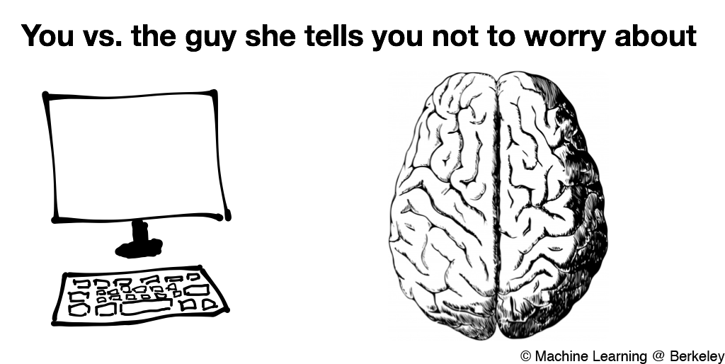
The perceptron mimics the function of neurons in machine learning algorithms. The perceptron is one of the oldest machine learning algorithms in existence. When it was first used in 1957 to perform rudimentary image recognition, the New York Times called it:
the embryo of an electronic computer that [the Navy] expects will be able to walk, talk, see, write, reproduce itself and be conscious of its existence.
We’re still a little far off from that, but the Times did recognize the potential of a perceptron. Perceptrons now form the basis for more complicated neural networks, which we’ll be talking about in the next post.
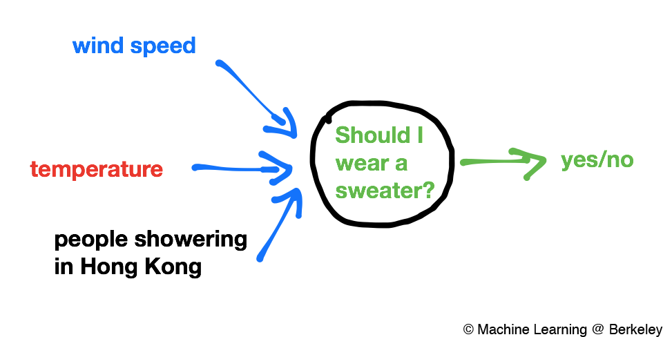
Like neurons, perceptrons take in several inputs and spit out an output. For example, a perceptron might take as input temperature and try to answer the question, “Should I wear a sweater today?” If the input temperature is below a certain threshold (say, 70˚F), the perceptron will output 1 (yes). If the temperature is above the threshold, the perceptron will output a 0 (no).

Of course, we could consider more variables than just temperature when deciding whether or not to wear a sweater. Like how a biological neuron typically can have more than one input electrical impulse, we can make our perceptrons have multiple inputs. In that case, we’ll have to also weight each input by a certain amount. If we were to use temperature, wind speed, and something completely random like the number of people showering in Hong Kong as our inputs, we would want to use different weights for each input. Temperature would probably have a negative weight, because the lower the temperature the more you should probably wear a sweater. Wind speed should have a positive weight, because the higher the wind speeds the more likely you will need to put on a sweater. And as for the number of people showering in Hong Kong, the weight should probably be zero (unless you normally factor in the number of people taking showers in Hong Kong into your decision making).
But someone from Canada might be very used to the cold, so their threshold for wearing a sweater might be a lower temperature than someone from, say, Australia. To express this, we use a bias to specify the threshold for the Canadian and the Australian. You can think of the bias as a measure of how difficult it is for the perceptron to say ‘yes’ or ‘no’.

The Canadian is fairly insensitive to cold temperatures, and thus has a low bias
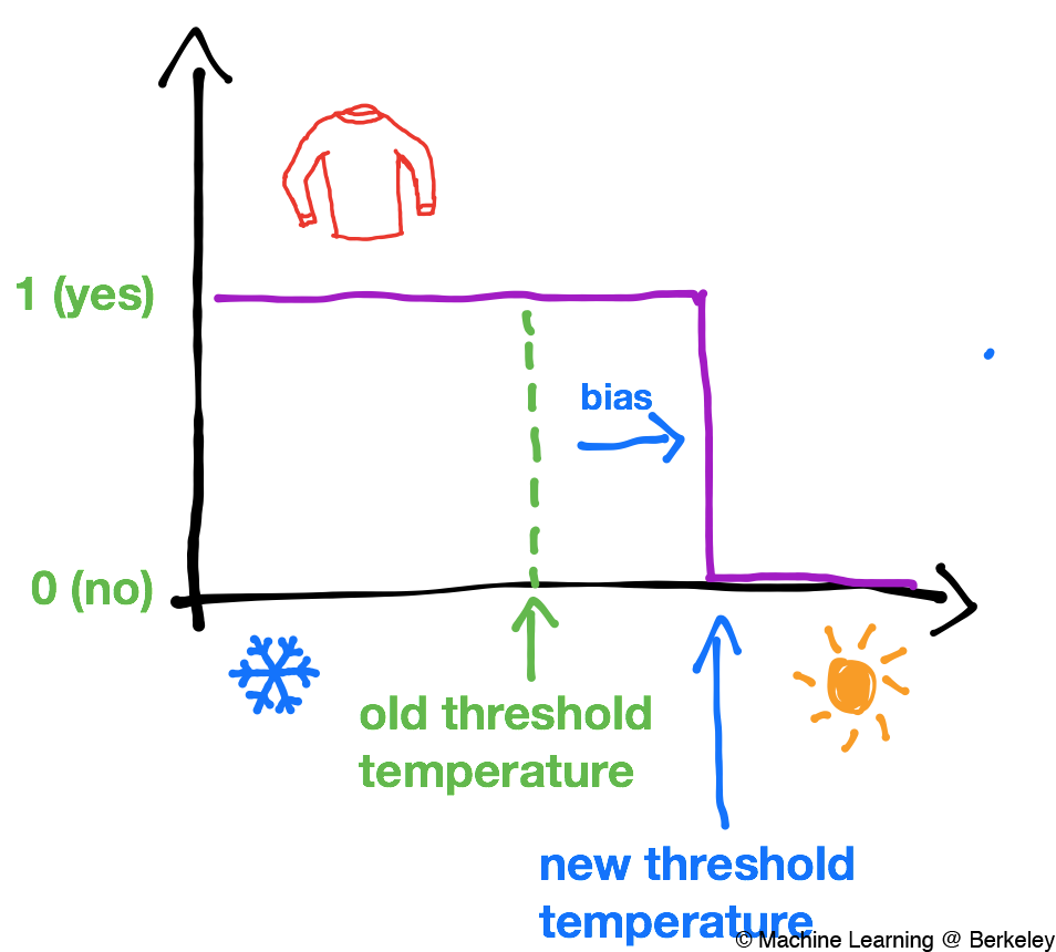
The Australian is biased towards hotter temperatures and thus has a higher threshold temperature
Logistic Regression
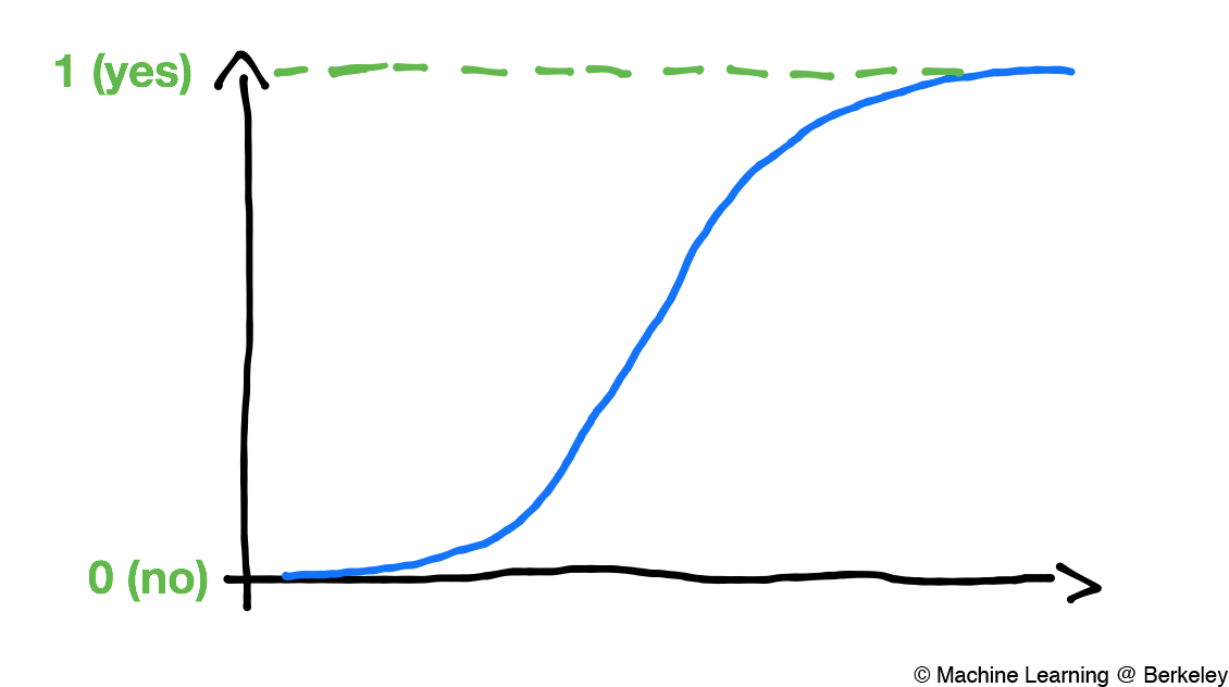
However, life is not as black and white as perceptrons indicate. There is uncertainty in just about anything, even choosing whether or not to put on a sweater. In reality, we don’t immediately put on a sweater the moment it drops below some predefined temperature. It’s more as if at any temperature we have a certain “chance” of putting on a sweater. Maybe at 45 F somebody will have a 95% chance of putting on a sweater, and at 60 F the same person will have a 30% chance of putting on a sweater.
To better model life’s complexities, we use logistic regression to find these probabilities. This involves fitting a logistic curve (like the one below) to our data. To do this, we again use gradient descent to choose the best parameters for the model. That is, we find parameters that minimize some cost function.
The general form of the logistic model is
where \(\theta\) is a vector of parameters, \(x\) is the input variables, and \(h\) is the model probabilities. For more information, we suggest you check out Andrew Ng’s notes on logistic regression.
Logistic regression and the perceptron algorithm are very similar to each other. It’s common to think of logistic regression as a kind of perceptron algorithm on steroids, in that a logistic model can predict probabilities while a perceptron can only predict yes or no. In fact, taking a logistic model and setting all values less than .5 to zero, and all values above .5 to one gives a very similar result to just the perceptron algorithm.
Support Vector Machines
Support vector machines, or SVMs for short, are a class of machine learning algorithms that have become incredibly popular in the past few years. They are based on a very intuitive idea. Here, we’ll introduce SVMs and go through the key ideas in the algorithm.
Margins
If you remember the section on classification from our last post, we classify data by drawing a line, called a decision boundary, to separate them.

Once we’ve drawn a decision boundary, we can find the margin for each datapoint. The margin for a single data point is the distance from that data point to the decision boundary.
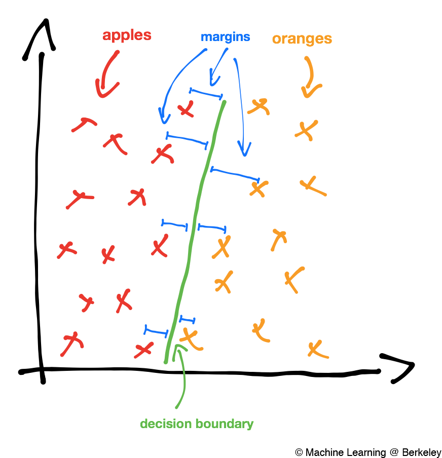
In a way, a margin is a way to determine how confident we are in our classification. If a data point has a large margin, and hence is very far away from the decision boundary we can be pretty confident about our prediction. However, if a data point has a very small margin, and is hence very close to the decision boundary then we probably aren’t as sure of our classification.
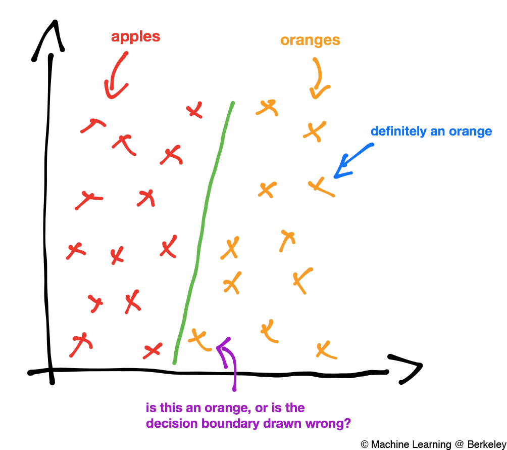
Now that we’ve defined margins, we can talk about support vectors. A support vector is a vector from the data point with the smallest margin to the decision boundary. In other words, it’s a vector between that data point that is closest to the decision boundary and the boundary itself. This vector, in fact, any margin, will be perpendicular to the decision boundary because the smallest distance between a point and a line is a perpendicular line.
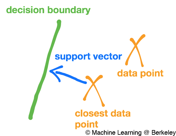
The idea behind a support vector machine is to classify data by drawing a decision boundary such that it maximizes the support vectors. By maximizing the support vectors, we’re also maximizing the margins in a data set, and thus the decision boundary is as far away as possible from the data points.
Linear Separability
If you’ve played around with the simulation enough, you’ll notice that sometimes the algorithm fails completely. This happens only when the data points aren’t linearly separable. Think of it this way: when you have a set of data points which you can’t draw a straight line to separate them with, then you have a linearly inseparable dataset, and since it’s impossible to draw a line to split them, then the SVM algorithm fails.
So how do we deal with linear inseparability? Turns out we can reformulate our optimization problem. Before, we wanted every single data point to be as far away (to the correct side) from the decision boundary as possible. Now, we’ll allow a data point to stray toward the wrong side of the boundary, but we’ll add a “cost” to that happening (remember cost functions from the last post?). This is something that happens very often in machine learning and is called regularization. It basically allows our model to be a bit more flexible when trying to classify the data. The cost of violating the decision boundaries can be as high or as low as we want it to be, and is controlled by something called the regularization parameter.
Mathematically, we implement regularization by adding a term to our cost function. For instance
\[C = C(\theta, x_i) + c\sum_{i} R_i(x_i)\]could be the regularized cost function, where C (the cost) is a function of all the parameters and all the training data, R is the regularization (or penalty) for each data point, and c is the regularization parameter. A large c would mean the penalty for violating the decision boundary would be very high, and vice versa.
This part is a bit mathy, which is why it’s hidden, but it’s also very fascinating. Now the SVMs shown so far can only make straight decision boundaries. But what if we wanted to classify data using a different kind of boundary? Well, that’s where kernels come in. Kernels are (loosely speaking) a fancy term for an inner product.
So why do we need kernels? It turns out that the SVM algorithm never depends on just a data point itself, but rather it depends on the inner product between data points. For that reason, we never need to know the coordinates of a data point, we only need to know the inner products between all the data points.
It turns out that for certain representations of data (or certain coordinate systems), it’s actually much easier to calculate the kernel than it is to calculate the actual data point. For example, we can use data points in an infinite dimensional space. As long as we have a way of computing the inner product, or the kernel, quickly. And luckily, there are ways to do this! One example of this is the Radial Basis Function kernel, which calculates the inner product for a certain infinite dimensional space. The form of the RBF kernel is
\[K(x, x') = e^{-\frac{||x-x’||}{2\sigma^2}}\]where x and x’ are the two data points in the original coordinate system, ||x-x’|| is the distance between the two points, and sigma is a parameter that controls the model’s behavior. The feature space for the RBF kernel is actually infinite, and would be completely unrepresentable completely in a computer, but using the kernel we can actually use SVMs in that feature space.
Another example of a kernel is the polynomial kernel, which takes the form
\[K(x, x') = (x^Tx'+c)^d\]where x and x' are the two data points, and c and d are parameters for the kernel. In this case, the feature space is not actually infinite, but the kernel is still helpful because it allows us to change our representation of the data.
Intuitively, you can think of a kernel as mapping a set data from one coordinate system to another coordinate system. In the original coordinate system the data may not be linearly seperable at all, whereas in the new coordinate system if we choose the correct kernel, we should get a set a data set is very easily linearly seperable.
Computationally intensive simulation! Press start to begin the simulation. (Unfortunately doesn't work on mobile). Left click to add red data point, shift-left click to add green data point. Click and drag to move the data points around. Use the sliders to adjust the regularization parameter (C), the sigma of the RBF kernel (must be in RBF kernel mode), and the C and Degree for the polynomial kernel (must be in polynomial kernel mode). Press 'k' to switch kernels. Press 'r' to reset the data points.
This simulation is an adaptation of Andrej Karpathy's SVM simulator which can be found here
SVM Simulation!
C = 1.0
RBF Kernel sigma = 1.0
Polynomial Kernel C = 0.0
Polynomial Kernel Degree = 2.0
Things to try with the simulator
- Use the linear kernel and set the regularization parameter (C) to 1.0e+6. Put two red data points and two green data points. Can the SVM classify linearly inseperable data? How about for other values of C?
- Try using the RBF kernel with different sigmas. Does the RBF kernel overfit or underfit the data?
- Try using different degrees polynomial kernels. Does the shape for a second degree polynomial kernel look familiar?
