Machine Learning Crash Course: Part 3

Neural networks are perhaps one of the most exciting recent developments in machine learning. Got a problem? Just throw a neural net at it. Want to make a self-driving car? Throw a neural net at it. Want to fly a helicopter? Throw a neural net at it. Curious about the digestive cycles of your sheep? Heck, throw a neural net at it. This extremely powerful algorithm holds much promise (but can also be a bit overhyped). In this article we’ll go through how a neural network actually works, and in a future article we’ll discuss some of the limitations of these seemingly magical tools.

The Biology

The biological brain is perhaps the most powerful and efficient computer that we know of. Compared to our complex organ, even our most powerful supercomputers are a joke. In 2014, Japanese researchers used a supercomputer to simulate just one second of human brain activity. It took 40 minutes and 9.9 million watts. As for the real thing? The little ball of grey matter in our skulls runs on only 20 watts, which translates to roughly one McChicken a day.

Neglecting a lot of details, biological neurons are cells that send and receive electrical impulses from other neurons that they are connected to. A neuron will only fire an electrical impulse when it receives impulses from other neurons that together are stronger than a certain threshold. Anything lower than that threshold and the neuron won’t do anything. Just what that threshold is depends on the chemical properties of the neuron in question and varies from neuron to neuron. Upon firing, an electrical impulse shoots out of the neuron and into more neurons downstream and the process continues. In the brain, billions of these interconnected neurons communicating with each other form the basis for consciousness, thought, and McChicken cravings.

The History

In the mid 1900’s, a couple of researchers came up with the idea of creating a “mathematical model” that would be based on how the brain works. They first created a model for a single neuron which imitated a real neuron’s outputs, inputs, and thresholds. The outputs of these single artificial neurons were then fed into even more artificial neurons, creating an entire artificial neural network.

There was just one problem: While researchers had created a model of the human brain, they had no way of teaching it anything. The artificial brain could be wired in whatever way researchers wanted, but the vast majority of these wirings didn’t create a brain that had any logical output at all. What was needed was a learning algorithm for their artificial brain.

It was not until the 1980’s that such an efficient learning algorithm was used on neural networks. The algorithm was called backpropagation, and finally allowed neural networks to be trained to do amazing things such as understanding speech and driving cars.

The Model (Overview)

Now that we know the basics of how the brain works and the history of neural networks, let’s look at what a neural network actually does. First off, we’ll think of our neural network as a black box, some machine whose inner workings we don’t really know about yet. We want this machine to take in some set number of numerical inputs (that we can choose) and spit out a set number of numerical outputs (that we can also choose).

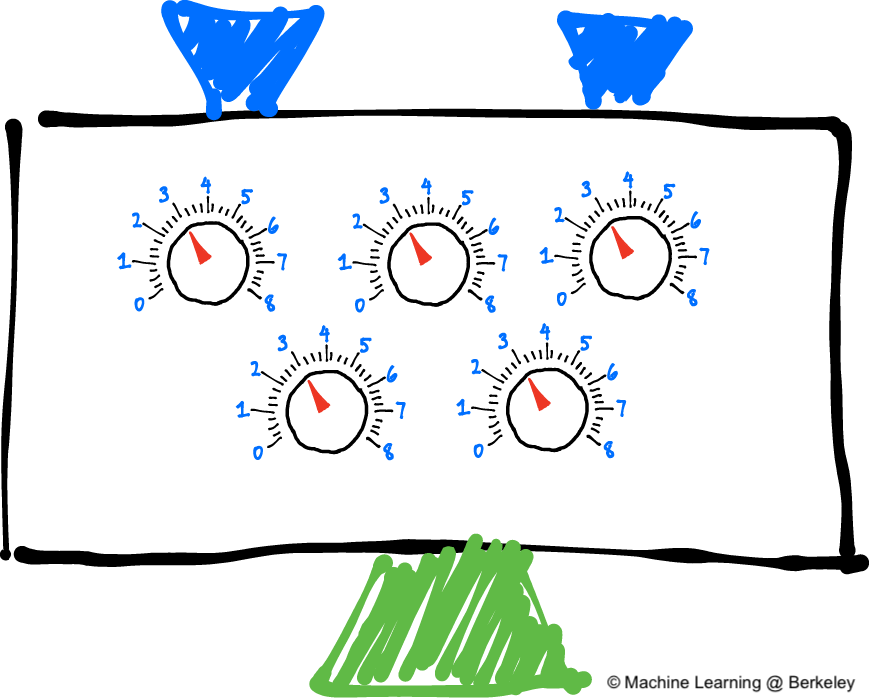
A neural network takes in some inputs, math happens, and some number of outputs pop out

For example, if we want to classify images (say apples and oranges) then we’d want the number of inputs to be the number of pixels in our images, and the number of outputs to be the number of categories we have (two for the case of apples and oranges). If we were trying to model housing prices then the number of inputs would be the number of features we have, such as location, number of bathrooms, and square footage, and the number of outputs would be just one, for the price of the house.

Our machine has inputs and outputs, but how do we control what inputs create what outputs? That is, how do we change the neural network so certain inputs (say an image of an apple) give the correct outputs (say a 0 for the probability of being an orange and a 1 for the probability of being an apple)? Well, we can add “knobs” to our machine to control the output for a given input. In machine learning lingo, these “knobs” are called the parameters of a neural network. If we tune these knobs to the correct place, then for any input we can get the output that we want.

Going back to our apples and oranges example, if we give our machine an image of an apple but it tells us it thinks it’s an orange then we can go ahead and adjust the knobs of our machine (in other words, tune the parameters) until the machine tells us it sees an apple. In essence, this is what it means to train a neural network and this is exactly what the backpropagation algorithm does.

The Model (Details)

Now that we know what a neural network should do and roughly how we can get it to learn, let’s peer inside the black box and talk about what is happening inside the network. To start, we’ll discuss what happens inside a single artificial neuron and build it up from there.

For those who have read our post on perceptrons, this will be very familiar material. That’s because a neuron in a neural network is basically a perceptron on steroids. Similar to a perceptron, a neuron takes in any number of numerical inputs and spits out just one output. To get to this output, the neuron calculates an intermediate value called \(s\) by multiplying each input by a different weight, adding them all together, and adding an additional number called the bias. In math: \(s = weight_{1}\times input_{1}+...+weight_{n}\times input_{n}+bias\)

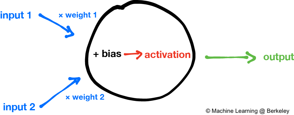
A neuron weights its inputs and then sums them up with a bias. An activation function is then applied, which produces the output for the neuron

Now each neuron could simply output \(s\), but that would be a bit boring as \(s\) is just a linear function, which makes it rather inflexible for modeling real-world data. What we want to do instead is to add one more step, called an activation function. An activation function is any function that takes in our \(s\) and gives the output of our neuron, called the activation. The perceptron that we described in the last post gave definitive yes/no answers using a blocky step function as its activation function.

For the step function, there is no way to tell how close you are to a “yes” or a “no”

However, using a step function makes training very difficult because there’s no way to tell whether the neural network is getting closer or farther from the correct answer. Imagine you are an ant that can only see things very close to you. You are on the higher part of the step function trying to get to the lower part of the step function. But because everything is so flat, you wouldn’t know how far away the “step” part of the step function is, or even in which direction it is. The “blocky” structure makes the step function a bad activation function for neural networks.

To make it easier to train a network, we’ll use a function that is smooth (in other words, a differentiable function). For example, we can use the sigmoid function, which looks something like this:

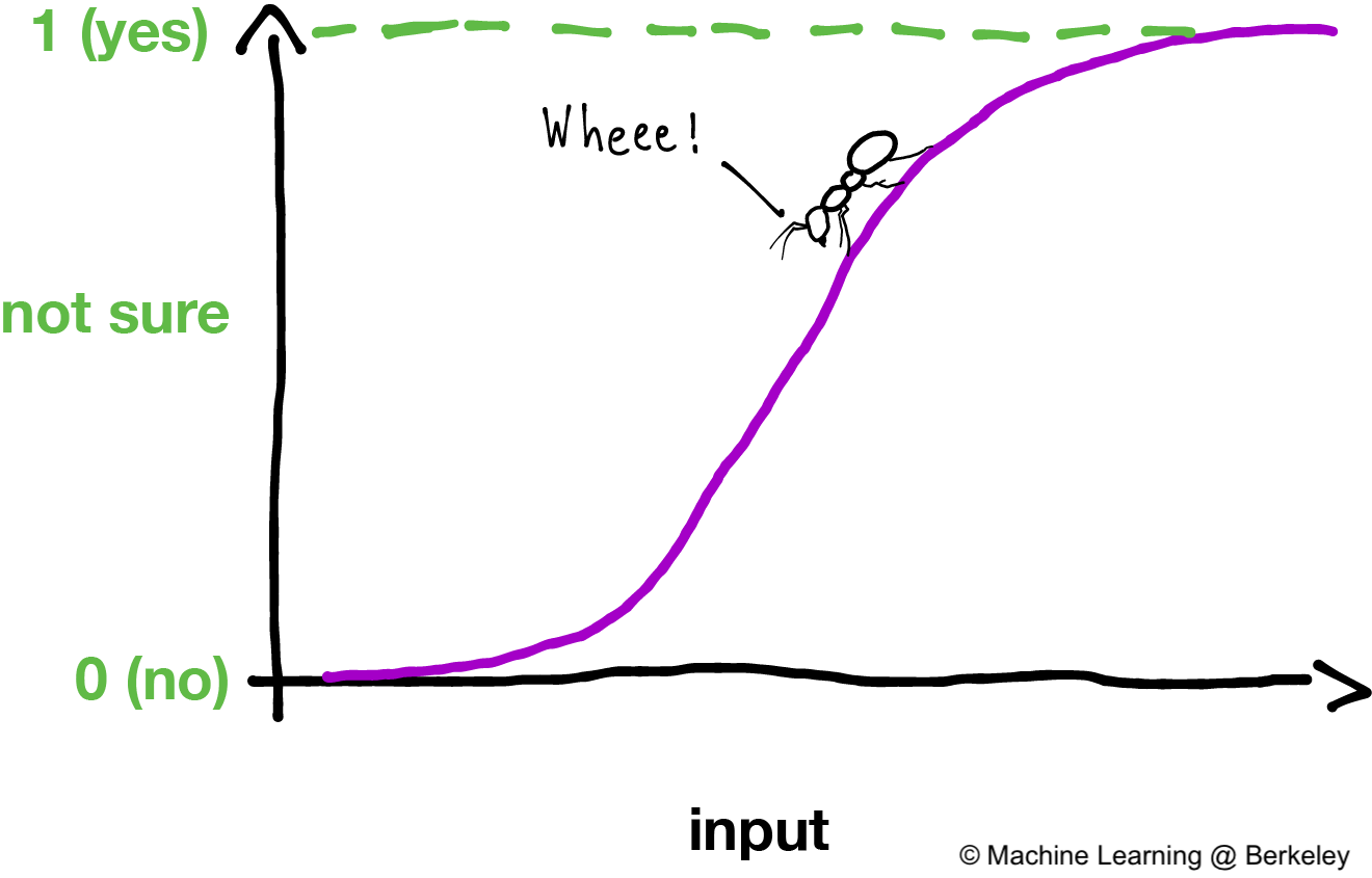
A sigmoid function is a nice activation function because it is smooth everywhere, making it easier to figure out if you're getting closer to the top

Going back to our ant analogy, an ant could figure out exactly which direction to go and how far to go just by checking in which direction and how much the graph slopes at its current location. Despite the fact that the ant can’t see the low part of the sigmoid function, it can get a rough idea of where it is by looking whether the part of the function it is standing on is sloping up or down.

Linking it all together

We wouldn’t have much of a network if we just had one neuron, would we? The secret to a neural network’s ability to make complex decisions lies in its internal structure of interconnected neurons. Just like how neurons in the brain are connected to each other, the output of one neuron becomes the input of another neuron, allowing the neurons to work together to come up with the correct answer.

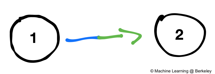
The output of neuron 1 (blue) becomes the input of neuron 2 (green)

Of course, we can’t just randomly connect neurons to each other and expect everything to work perfectly. The design of a neural network is based on the way our brains process data by structuring neurons into groups of computational “units.” For example, the human visual cortex consists of 5 distinct sections called V1, V2, V3, V4, and V5. Visual stimuli travels from the retina to V1 where low-level details such as edges and colors are picked out. The information generated by V1 then travels to V2, and then V3 and so on, with each cortex processing progressively more and more complicated information.

Neural networks are composed of layers, with connections from one layer to the next layer

Artificial neural network are composed of layers of artificial neurons in a similar way. In general, there are three types of layers: an input layer, one or more hidden layers, and an output layer. The input layer (on the very left) will take on values of whatever the input is to the the neural network. Notice that we can have our network take any number of inputs by changing the number of neurons in the input layer. Neat!

Similarly, the output of the output layer (on the very right) will be the output of the whole neural network, and we can change the number of neurons in the output layer to match the number of outputs we want from our network.

Between the input layer and the output layer are hidden layers. The optimal number of hidden layers is the subject of much discussion, but the short answer is that it’s completely up to whoever builds the network. For simplicity, we’ll talk about a network with one hidden layer.

Finally, each layer is fully connected to the one before it and after it. This means the output of a single neuron in a layer connects to (or is the input of) every neuron in the next layer, because the information that a neuron provides in one layer could be useful to any neuron in the next layer. Between each connection is a weight that the output is weighted by. Let’s go through a visual example:

❮ ❯

How a Neural Network “Works”

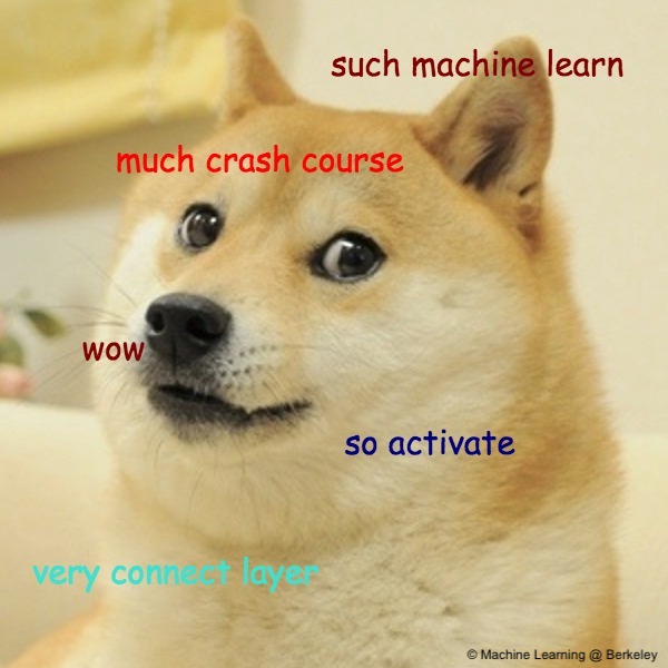
You've been visited by ML-Doge! Please don't overfit!

Say you’re trying to recognize Doge. Do the pink and green blobs(flowers) in the background matter when trying to identify the main object in the picture? Probably not, so that information can probably be discarded.

So what information is relevant? Well, the object has lines of dark and white pixels that indicate fur, ovals that indicate eyes, triangular things that are probably ears, and a big dark triangle-oval patch that seems to be a nose.

Many people will probably immediately recognize the object as a dog, but what gives it away? Fur, eyes, ears, and nose are all indications, but they must be considered together in order to figure out that the object is a dog.

We can visualize this thought process with various neurons tasked with identifying increasingly abstract objects in the image:

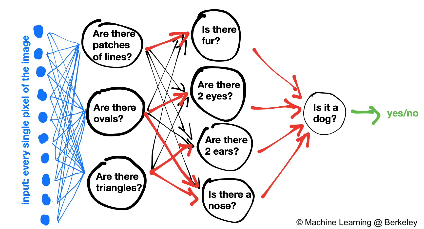
How someone might identify a dog. Important inputs that are given a lot of weight are highlighted in red.

Notice how the neurons are organized into layers, where the further right the neurons are, the more abstract the input? In other words, the neurons on the left ask questions about general shapes and lines, whereas the neurons on the right ask questions about objects such as eyes or fur. Trained neural networks function in a very similar way, although they arrive at this conclusion after training with a lot of data. No one explicitly tells the network to identify dogs in the fashion described above.

The above example just provides a rough, slightly inaccurate but conceptual understanding of what’s really happening under the hood to make the reasons behind the design of a neural network more clear. You can see some examples of what neurons “actually” see here. It takes raw data and refines it with math until it has the answer that it needs.

Training

Okay, we’ve put it off for long enough! Let’s talk about the real meat of machine learning: The training!

At its very core, training a neural network just means adjusting the parameters (i.e., the weights and biases) until our network outputs the correct answer (or at least something sufficiently close to it). Precisely how to adjust the parameters for each neuron in the network is one of the reasons why machine learning is such a complicated field of study. We’ve already covered the general strategy for adjusting the parameters in the Regression section of our first tutorial and you can read about it there, but the gist of it is that you need to specify a cost function that quantifies how “wrong” your neural network is by outputting large values for very wrong answers and small values for more correct answers (you want the cost function to get as close to zero as possible).

For example, if we feed a neural network an image of an apple and it tells us it sees an orange, then the cost for that particular example would be high. The term “cost” comes from the fact that you can think of a neural network with a high cost (and therefore many wrong answers) as bad, or expensive, and vice versa. To ensure that a neural network’s correct answer isn’t just some fluke, networks are typically trained on thousands upon thousands of training examples. Once we have a cost function and many training examples, we can then perform gradient descent to minimize the cost function by adjusting our parameters.

To review, gradient descent is a way to find the minimum of a function. In the case of a neural network, the function that we want to minimize is the cost function. Gradient descent does this by adjusting the parameters of the network such that we get a lower value from the cost function than before. In a sense, gradient descent “moves” downhill whenever possible like an ant feeling out the slope of the terrain. And each time it moves downhill, the gradient descent “saves” its progress by updating the weights and biases in each neuron. Eventually, gradient descent will have found the very bottom of the cost function.

Backpropagation

Of course, gradient descent needs to know which direction is “downhill” in order to work. Using our ant analogy, an ant sitting on the cost function only knows which way to go because the part of the function it is standing on is sloped. Remember, it can’t see very far, and certainly not far enough to see where the minimum actually is. The ant’s best bet is to go the direction that is sloping downhill the most.

In math terms, these slopes are derivatives. Now if you suddenly felt a panic attack settling in upon reading the word “derivative” (or if you have absolutely no idea what a derivative is) don’t worry. We’ve tried our best to make this whole section completely understandable through just intuition. On the other hand, if you suddenly felt a rush of exhilaration we encourage you to go tackle the collapsible sections at the end of this article where we derive the backpropagation formulas.

The whole point of backpropagation is to find these slopes to help gradient descent work. There is in fact a different slope we need for each of our parameters. That is, going back to our machine analogy you can imagine yourself turning the knob for single parameter and watching the cost function go up or down. The slope for a particular parameter will tell you which way to turn the knob to make the cost function go down. Once we find out which way to turn each of the knobs (in other words, once we have the derivative of the cost with respect to each of the parameters: the weights and biases) we can turn each of the knobs in the correct direction a tiny bit.

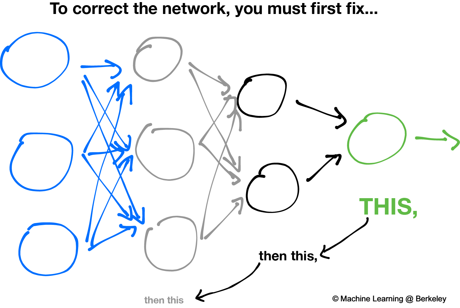
To introduce backpropagation, let’s start with another analogy. Don’t worry if you can’t see how this has anything to do with backpropagation (trust us, it does). Let’s say you want to push a marble off a table with a line of dominos. During your first try, you discover that the dominos were placed too far from the marble so that the last domino falls short of the marble. What do you do to fix this? You can’t move the marble, since it needs to fall off the table, so you take the domino closest to the marble and place it closer. Subsequently, you’ll need to take the second to last domino and place it closer to the one you just moved, and so on until you move the entire line of dominos closer to the marble, starting with the domino closest to the marble.

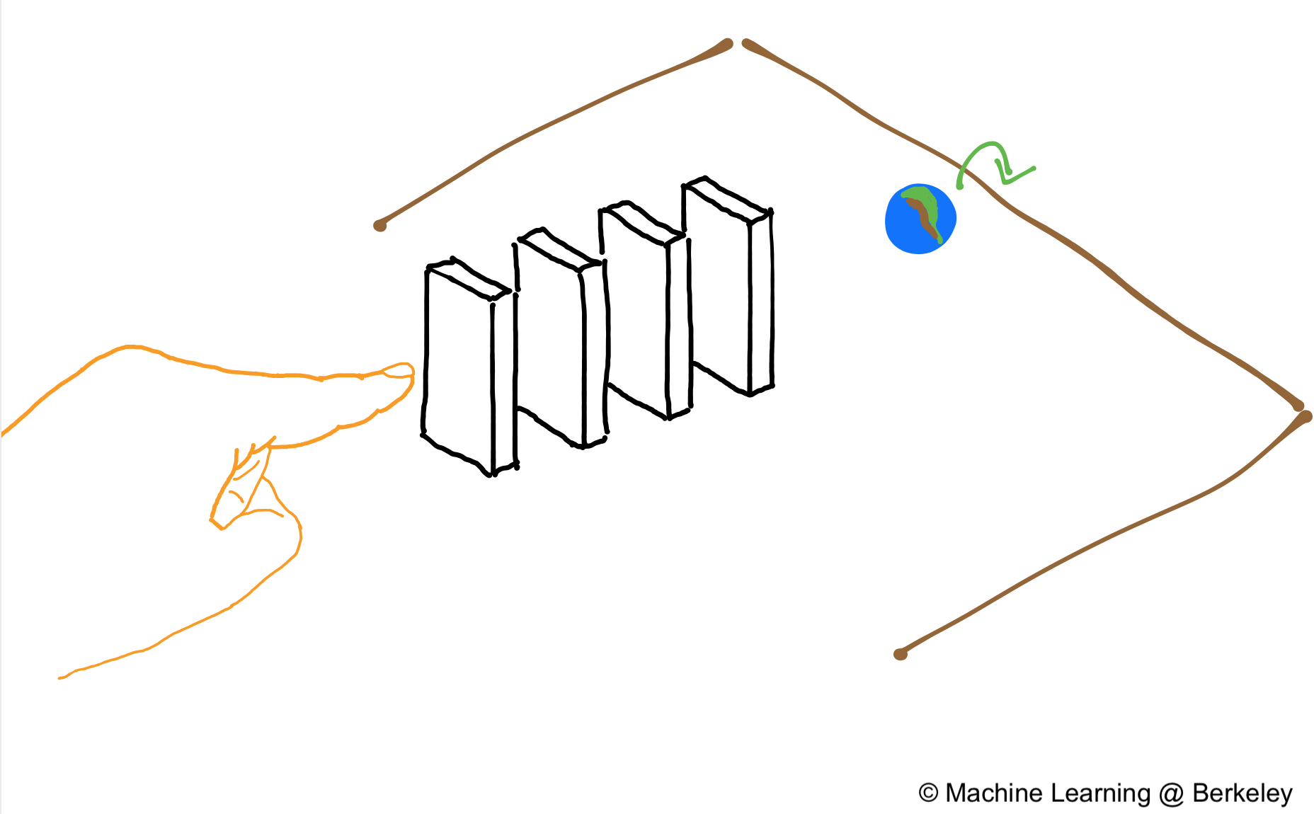
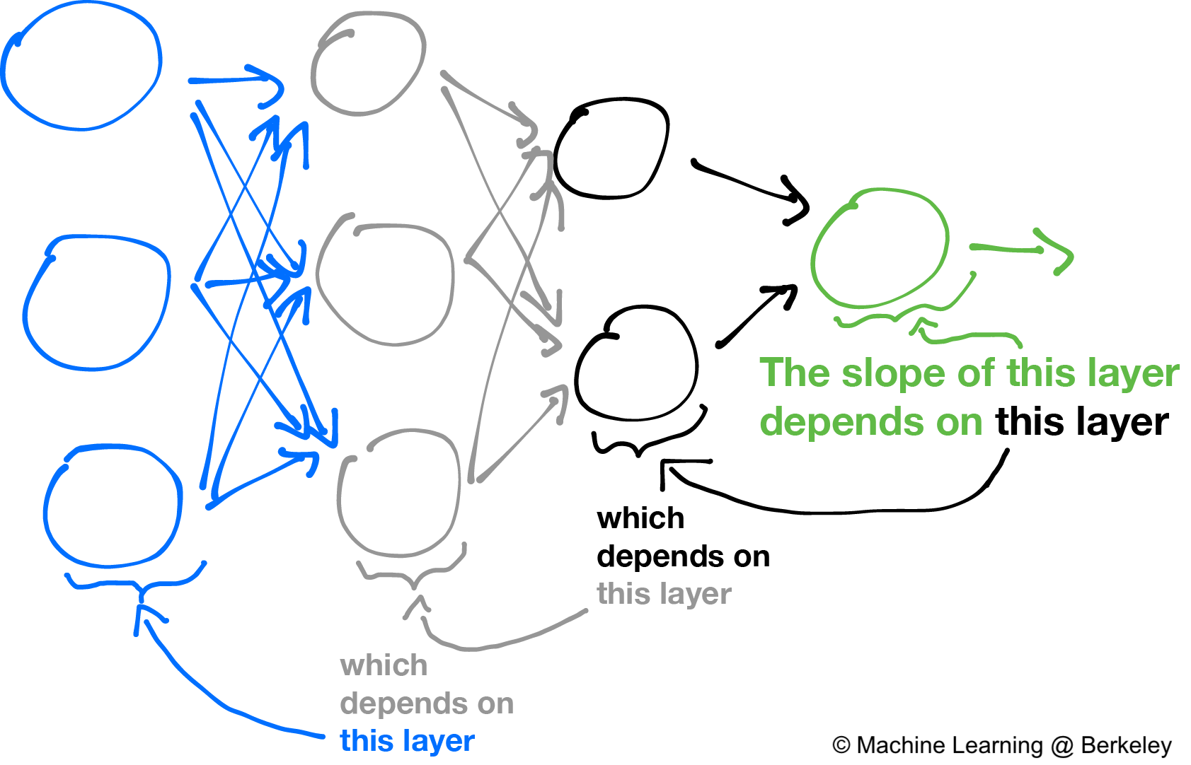
Backpropagation works in a similar way. When the neural network outputs the wrong answer (doesn’t push the marble off the table), you find the slopes of the output layer (the domino closest to the marble) first because it was the direct cause of the incorrect answer. And since the output layer depends on the hidden layer, you’ll have to fix that too by finding the slopes and using gradient descent. Eventually you’ll work your way back to the hidden layer closest to the input layer.

It turns out that once we calculate the slopes of a given layer, we can easily find the slopes of a previous layer. Intuitively, this makes sense because changing the parameters in one layer will affect the outputs of the next layer which will affect the outputs of the next layer, and so on until the cost function itself is affected. Therefore we need to know how all future layers will affect the cost function before we know how a specific layer will affect the cost function.

Thus, we easily calculate the slopes of the last layer, and then the second to last layer, and end up working backwards until we reach the first, input layer. This is the namesake for our algorithm: “backpropagation.” We calculate slopes by starting from the back and propagating our algorithm backwards through the neural network until we get all the slopes for gradient descent.

That, in a nutshell, is the backpropagation algorithm—the very reason cars can drive themselves, Siri can recognize your voice, and computers can read your checks. Don’t worry if you don’t understand everything immediately. For most people it takes more than a few read-throughs to fully understand what is happening. For those of you who feel affronted that the math has been skipped over, feel free to check out the next section. We first introduce notation to describe neural networks in an elegant way using matrices. Then we derive the rules of backpropagation. Cheers!

Backpropagation

Feedforward in Matrix Notation

To use gradient descent we need to find the derivatives of the cost function with respect to each of the parameters. In order to do this, let’s formalize our picture of a neural network in the language of matrices and vectors. In particular, our goals is to write down the feedforward step, that is, turning one layer’s outputs into the next layer’s outputs.

Why matrices and vectors though? Why go through all the trouble? Matrices and vectors give us a “global” view of what is happening in a neural network. That’s because whole layers can be represented by vectors, and operations on layers (such as applying weights and summing) can be represented with matrices. This global view of looking at all the neurons in a layer at once, as opposed to a “local” view looking at only the individual neurons in each layer, allows us to write equations in a very concise, and arguably elegant manner.

Let’s begin by writing our inputs as a column vector, called \(a^1\). So if we have \(n\) inputs, then our input vector would essentially be a \(1 \times n\) dimensional matrix. Something like this:

\[a^1 = \begin{bmatrix} i_1 \\ i_2 \\ \vdots \\ i_n \end{bmatrix}\]

Now be careful. The superscript \(1\) is not an exponent (if it were it would be quite redundant). Rather it is used to indicate that the vector is associated with the first layer of our network, in other words, the input layer. We choose the letter \(a\) because we can think of the inputs as being the activations (aka the outputs) of the first layer of neurons. You may have already guessed, but we’re going to be calling the vector of activations for the \(l^{th}\) layer \(a^l\). And if we have \(L\) layers, then \(a^L\) (that is, the activations of the very last layer, the output layer) will be the output of our entire neural network. Every \(a^l\) will have a different dimension depending on how many neurons are in each layer.

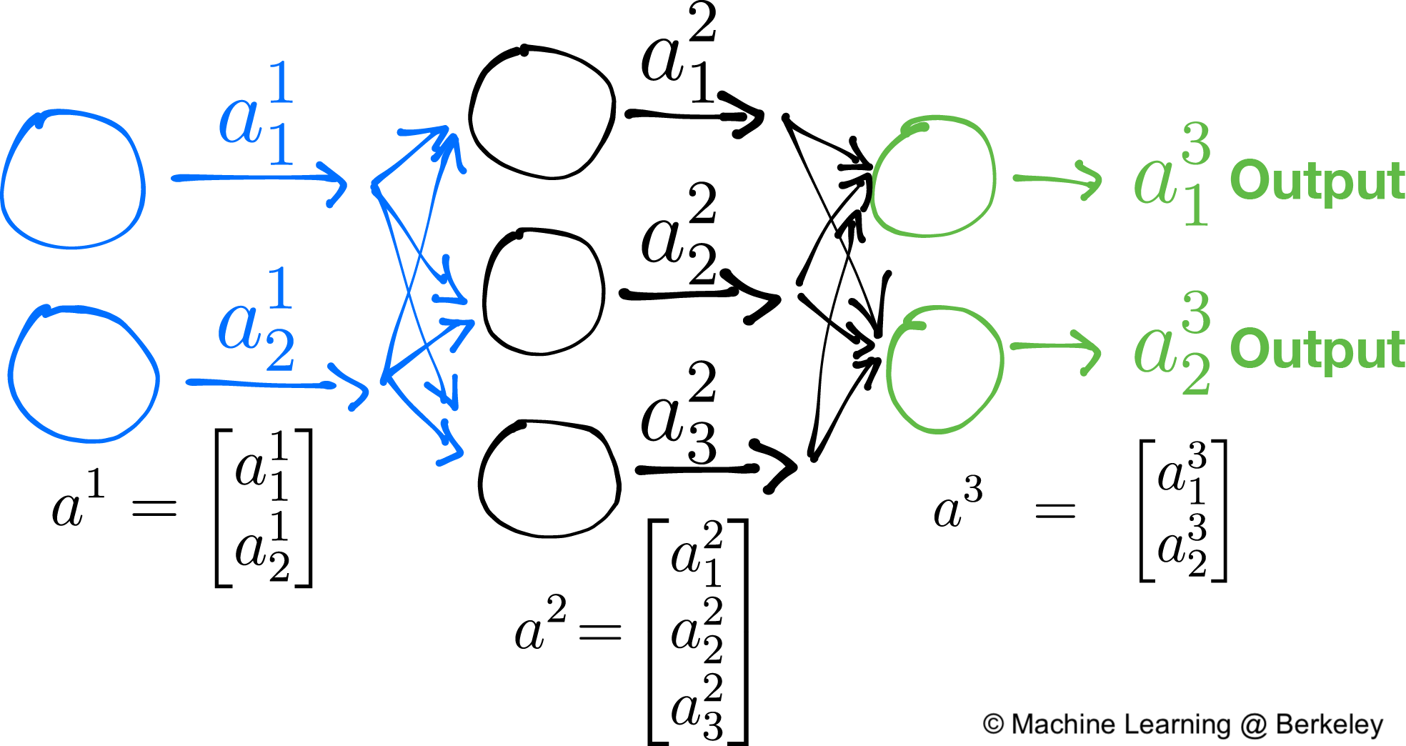
Now let’s figure out how to write the weights in matrix notation. Of course, we could just throw all the weights into some matrix and call it a day, but let’s be a bit more clever about it. In particular, let’s take advantage of matrix multiplication. We’ll define a \(N \times 1\) dimensional vector to be the weights vector from a previous layer to a single neuron in the next layer, where \(N\) would be the number of neurons in the previous layer (all of this seemingly arbitrary notation will pay off in the end, we promise). Let’s call this vector \(w^l_k\) for the \(k^{th}\) neuron in the \(l^{th}\) layer.

The weights of the vectors pointing to the red neuron would be referred to as \(w^3_1\), where \(w^3_1 = \begin{bmatrix} w^3_{11} \\ w^3_{12} \\ w^3_{13} \end{bmatrix}\)

Notice now that for the \(k^{th}\) neuron in the \(l^{th}\) layer, we can get its weighted sum of its inputs, called \(z^l_k\) (where \(l\) is the layer and \(k\) is the \(k^{th}\) neuron) by taking the dot product between \(a^{l-1}\) and \(w^l_k\).

What’s more, we can actually write out a weight matrix for each layer, where each row in the matrix is a \(w^l_k\). Call this matrix \(w^l\):

\[w^l = \begin{bmatrix} \cdots w^l_1 \cdots \\ \cdots w^l_2 \cdots \\ \vdots \\ \cdots w^l_n \cdots \end{bmatrix}\]

Notice that this takes advantage of the definition of matrix multiplication in that \(w^la^{l-1}\) gives a vector of the weighted inputs for each neuron, which we’ll call \(z^l\).

\[w^la^{l-1} = \begin{bmatrix} \cdots w^l_1 \cdots \\ \cdots w^l_2 \cdots \\ \vdots \\ \cdots w^l_n \cdots \end{bmatrix} \begin{bmatrix} a^l_1 \\ \vdots \\ a^l_m \end{bmatrix}= \begin{bmatrix} w^l_1 \cdot a^{l-1} \\ w^l_2 \cdot a^{l-1} \\ \vdots \\ w^l_n \cdot a^{l-1} \end{bmatrix} = \begin{bmatrix} z^l_1 \\ z^l_2 \\ \vdots \\ z^l_n \end{bmatrix} = z^l\]

(where there’s \(n\) neurons in the \(l^{th}\) layer and \(m\) neurons in the \((l-1)^{th}\) layer)

Each layer \(l\), with \(n\) neurons, also has a bias vector:

\[b^l = \begin{bmatrix} b^l_1 \\ b^l_2 \\ \vdots \\ b^l_n \end{bmatrix}\]

We can add this vector to our weighted sums vector, \(z^l\), which should also be \(1 \times n\) dimensional, to get \(s^l\). \(s^l\) here can be interpreted as the “layer-level” view of the “neuron-level” statement \(s = weight_{1}\times input_{1}+...+weight_{n}\times input_{n}+bias\) from above.

Now that we have \(s^l\), we can apply our activation function to it. Above, we introduced the sigmoid function as our activation function, but in fact any differentiable function can be used as our activation function, granted some are better than others (common ones include ReLU, tanh, and arctan). To account for this, we’ll use \(f\) to represent our activation function.

So to apply \(f\) to our \(s^l\) vector, we simply write \(f(s^l)\), which means applying \(f\) to each of the elements in the \(s^l\) vector.

To do a feedforward step, we first multiply the output of a layer by the weight matrix, add the bias vector, and then apply the activation function

Backpropagation

The whole point of backpropagation is to find the derivatives of the cost function with respect to all of the weights and biases in a neural network. In mathematical notation, we want:

\[\frac{\partial J}{\partial w^l_{jk}}, \frac{\partial J}{\partial b^l_{j}}\]

Where:

• \(w^l_{jk}\) is the weight from the \(k^{th}\) neuron in the \((l-1)^{th}\) layer to the \(j^{th}\) neuron in the \(l^{th}\) layer
• \(b^l_{j}\) is the bias for the \(j^{th}\) neuron in the \(l^{th}\) layer
• \(J\) is the cost function
• and taking the derivative of a matrix means taking the derivative of the elements

While this may seem like a daunting task at first, it turns out that the only tool we really need is our good friend chain rule (if you haven’t met it already, allow us to introduce you). By blindly throwing the chain rule at our cost function, we’ll eventually be able to stumble upon the derivatives that we want. When in doubt, chain rule!

First off, let’s talk about the cost function. Our assumption is that the cost function is some function of the outputs of the neural network and our training examples. So in general our cost function is \(J(a^L_1, a^L_2, \dots, a^L_m, y)\) where \(L\) represents the last layer which has \(m\) output neurons, and \(y\) represents our training data. For one, this should seem pretty intuitive for our cost function, after all the cost function should probably only be a function of the outputs of our algorithm (and our training examples).

Also, notice that any \(a^l\) is in turn a function of \(s^{l}\), and each \(s^l\) is in turn a function of all the \(w^l_{jk}\) and \(b^l_j\) in the layer. Having a cost function of this form makes it possible to use the chain rule very efficiently.

Now just one more thing before we start chain ruling away. To make our derivation a bit easier we’re going to calculate an intermediate value

\[\delta^l_j \equiv \frac{\partial J}{\partial s^l_j}\]

which is the rate of change of the cost function with respect to the \(j^{th}\) neuron in the \(l^{th}\) layer.

From this \(\delta^l_j\) we will be able to chain rule our way to the derivatives that we want. Namely:

\[\frac{\partial J}{\partial w^l_{jk}}, \frac{\partial J}{\partial b^l_{j}}\]

Alright, enough talk. Let’s (finally) start chain ruling. By using chain rule, we find that

\[\delta^l_j = \frac{\partial J}{\partial s^l_j} = \sum_k \frac{\partial J}{\partial a^l_k} \frac{\partial a^l_k}{\partial s^l_j}\]

We can apply the multivariate chain rule because \(J\) is a function of \((a^l_1, a^l_2, \dots, a^l_m)\), and each \(a^l_i\) is in turn a function of \((s^l_1, s^l_2, \dots, s^l_m)\). Actually, each \(a^l_i\) is a function of just \(s^l_i\). Namely \(a^l_i = \sigma ( s^l_i )\). Now this means \(\frac{\partial a^l_k}{\partial s^l_j}\) will be zero unless \(k=j\), in which case \(\frac{\partial a^l_k}{\partial s^l_j}\) will be \(\sigma’(s^l_j)\). Thus our expression for \(\delta^l_j\) simplifies to

\[\delta^l_j = \frac{\partial J}{\partial a^l_j} \sigma’(s^l_j)\]

Now for the actual “backpropagation” part of the algorithm. We’ll use chain rule to derive an expression for \(\delta^l\) from \(\delta^{l+1}\). In words, this means we will have a way of finding deltas in one layer from the deltas in the next layer. Once we figure out how to do this, we can just start from the very end layer of a neural network and work our way backwards finding all the deltas.

Alright, let’s chain rule this guy out. We start with

\[\delta^l_j \equiv \frac{\partial J}{\partial s^l_j}\]

and with chain rule we get

\[\delta^l_j = \sum_k \frac{\partial J}{\partial s^{l+1}_k} \frac{\partial s^{l+1}_k}{\partial z^l_j}\]

Again, we can apply the chain rule here because \(J\) is some function of \((s^{l+1}_1, s^{l+1}_2, \dots, s^{l+1}_n)\).

And also \(s^{l+1}_k\) is in turn a function of \((s^l_1, s^l_2, \dots, s^l_m)\). Essentially, what we’re saying is that the activations of one layer are a function of the activations of the previous layer.

Now notice \(\frac{\partial J}{\partial s^{l+1}_k}\) is actually \(\delta^{l+1}_k\). Substituting we get

\[\delta^l_j = \sum_k \frac{\partial s^{l+1}_k}{\partial s^l_j} \delta^{l+1}_k\]

Turns out we can simplify the \(\frac{\partial s^{l+1}_k}{\partial s^l_j}\) a bit more. Let’s explicitly write out \(s^{l+1}_k\):

\[s^{l+1}_k = \sum_j w^{l+1}_{kj} a^l_j + b^{l+1}_k = \sum_j w^{l+1}_{kj} \sigma(s^l_j) + b^{l+1}_k\]

The derivative of this with respect to \(s^l_j\) is

\[\frac{\partial s^{l+1}_k}{\partial s^l_j} = w^{l+1}_{kj} \sigma’(s^l_j)\]

Substituting into our expression for delta, we get

\[\delta^l_j = \sum_k w^{l+1}_{kj} \delta^{l+1}_k \sigma’(s^l_j)\]

Now, finally we have expressions to find the deltas of all the layers. Now how exactly do we actually get

\[\frac{\partial J}{\partial w^l_{jk}}, \frac{\partial J}{\partial b^l_{j}}\]

from these deltas?

You can probably guess by now; we’re going to chain rule them out!

Let’s start with \(\frac{\partial J}{\partial b^l_{j}}\). Using our trusty chain rule, we get

\[\frac{\partial J}{\partial b^l_{j}} = \frac{\partial J}{\partial s^l_j} \frac{\partial s^l_j}{\partial b^l_j}\]

By definition, \(\delta^l_j \equiv \frac{\partial J}{\partial s^l_j}\), and writing out \(s^l_j\) explicitly, we get

\[s^l_j = \sum_k w^l_{jk} a^{l-1}_k + b^l_j\]

Differentiating with respect to \(b^l_j\), we simply get \(1\). Thus, substituting these two expressions, our equation for the bias derivative is

\[\frac{\partial J}{\partial b^l_j} = \delta^l_j\]

The weight derivative is found in a similar manner. By chain ruling we get

\[\frac{\partial J}{\partial w^l_{jk}} = \frac{\partial J}{\partial s^l_j} \frac{\partial s^l_j}{\partial w^l_{jk}}\]

Again, the first term is the delta of the \(l^{th}\) layer. The second term we can find be differentiating our explicit formula for \(s^l_j\)

\[s^l_j = \sum_k w^l_{jk} a^{l-1}_k + b^l_j\]

Differentiating with respect to \(w^l_{jk}\), we get

\[\frac{\partial s^l_j}{\partial w^l_{jk}} = a^{l-1}_k\]

Substituting we get

\[\frac{\partial J}{\partial w^l_{jk}} = a^{l-1}_k \delta^l_j\]

which is what we want!

So in conclusion, there are really four main equations in the backpropagation algorithm:

• An equation to find the delta of the last layer:

\[\delta^l_j = \frac{\partial J}{\partial a^l_j} \sigma’(s^l_j)\]

• An equation to find the deltas of a layer from the deltas of the next layer (the backpropagation step):

\[\delta^l_j = \sum_k w^{l+1}_{kj} \delta^{l+1}_k \sigma’(s^l_j)\]

• An equation to find the bias derivatives from the deltas:

\[\frac{\partial J}{\partial b^l_j} = \delta^l_j\]

• And an equation to find the weight derivatives from the deltas:

\[\frac{\partial J}{\partial w^l_{jk}} = a^{l-1}_k \delta^l_j\]

These equations combined allow us to find the derivatives of a neural network, and in turn form the basis for a wide variety of neural network based algorithms. They find application in everything from helicopter auto-pilots, stock market prediction, disease diagnosis, and fraud detection. These are, of course, highly non-trivial applications so don’t be worried if you don’t understand these equations completely at first. True understanding will take time and practice with these equations.*

*Much of this section was shamelessly lifted from the amazing explanation of backpropagation Michael Nielsen gives in his great book Neural Networks and Deep Learning. As such, if you want more practice with the equations or want to read about backpropagation from a different perspective, we highly encourage you to check it out!

So far in this tutorial series we’ve talked about linear regression, logistic regression, the perceptron algorithm, and SVMs. These models are very effective and have solved some amazing problems. But at the same time, they are also very limited. For example linear regression requires the dataset to be, well, linear. And the perceptron algorithm and logistic regression can only draw a line through a dataset. Even SVMs are sensitive to what kernel is used.

Neural networks, however, gives us a framework that minimizes the drawbacks of these problems. Their adaptability, effectiveness, and efficiency have transformed the world and solved some of the most intractable problems that have stalled progress in many industries. Yet we know surprisingly little about this revolutionary tool. There is a lot of ongoing research into neural networks, and the coming years are sure to hold many more revolutionary discoveries.