
Machine Learning Crash Course: Part 5 - Decision Trees and Ensemble Models
26 Dec 2017 | Shannon Shih and Pravin RavishankerTrees are great. They provide food, air, shade, and all the other good stuff we enjoy in life. Decision trees, however, are even cooler. True to their name, decision trees allow us to figure out what to do with all the great data we have in life.
Like it or not, you have been working with decision trees your entire life. When you say, “If it’s raining, I will bring an umbrella,” you’ve just constructed a simple decision tree.
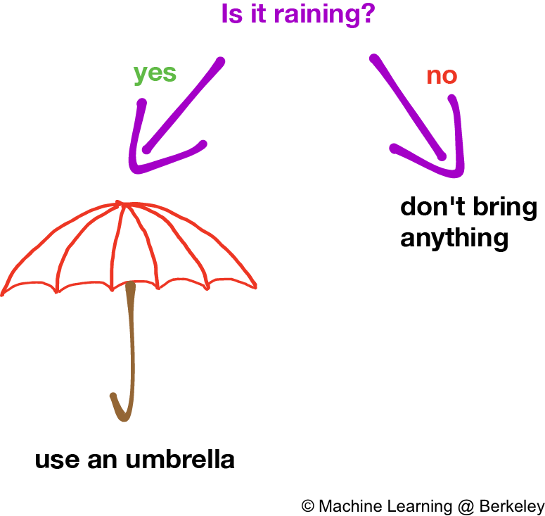
It’s a pretty small tree, and doesn’t account for all situations. Likewise, this simplistic decision making process won’t work very well in the real world. What if it’s windy? “If it’s raining and isn’t too windy,” you’ll say. “I will bring an umbrella. Otherwise, I will bring a rain jacket.”
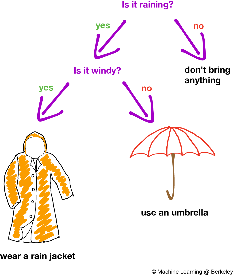
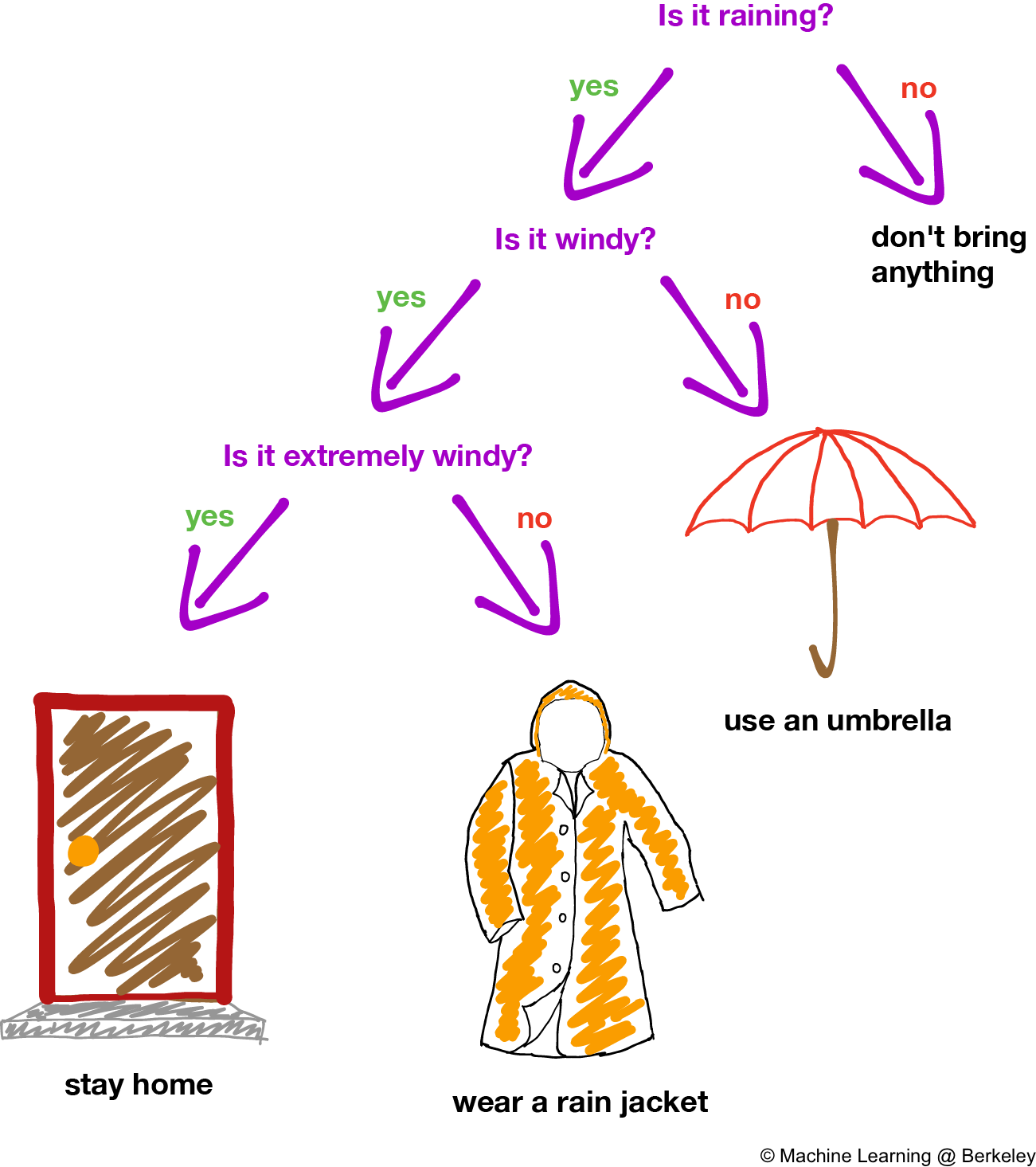
Better. We’ve added some leaves that represent the different choices we can make, and the branches of the tree represent “yes” and “no”. Although the decision tree represented above resembles an upside-down tree, it’s starting to look large enough to handle more situations. But what if the wind is extremely strong, like a hurricane? Rain jackets won’t do much good, as this guy found out (don’t try this at home):
Probably best to stay inside then.
Our tree’s starting to grow bigger, but what if it’s snowing? Or hailing? Our decision tree will need to grow a lot more in order to flourish in our complicated, rainy planet.
Easy to understand? Good, because simplicity is one of the biggest advantages of decision trees. Decision trees are very interpretable and understandable—they allow people to see exactly how the computer arrived at its current conclusion. To make a prediction on a new observation, we first find out which region that observation belongs to and then return either the mean of the data in that region if we’re predicting a number, or the most common labeled value in that region if we’re classifying things.
But there are some major disadvantages of decision trees. Although they are intuitive and interpretable, decision trees by themselves do not have the same level of predictive accuracy as some other popular machine learning algorithms. This is because classification and regression decision trees tend to make overly complicated decision boundaries, resulting in increased model variance that leads to overfitting. This in turn leads to more erratic predictions and increased error on unfamiliar data. In practice, however, we can use pruning algorithms to reduce the depth and complexity of the tree by removing nodes (i.e. questions) larger than a certain depth so that the decision tree does not overfit to the training data.
Decision Trees
Classification
Let’s say we wanted to classify different species of iris flowers (Iris Setosa, Iris Versicolour, Iris Virginica) given 4 quantities: the width and length of the flower’s sepal (the leaves that used to make up the flower bud), as well as the width and length of the flower’s petals. What kinds of questions should we ask in order to construct a good decision tree?
Say we pick a particular variable, such as flower petal length, and a corresponding value of that particular variable, such as 2.45 cm to reduce the number of possible species that some particular iris could be. Now we can divide all the training data into two groups: data points for which flower petal length is smaller than or equal to 2.45 cm, and the set of all data points for which flower petal length is greater than 2.45 cm. By choosing more variables and values, we can divide the data into different categories, then find out what species each category corresponds to.
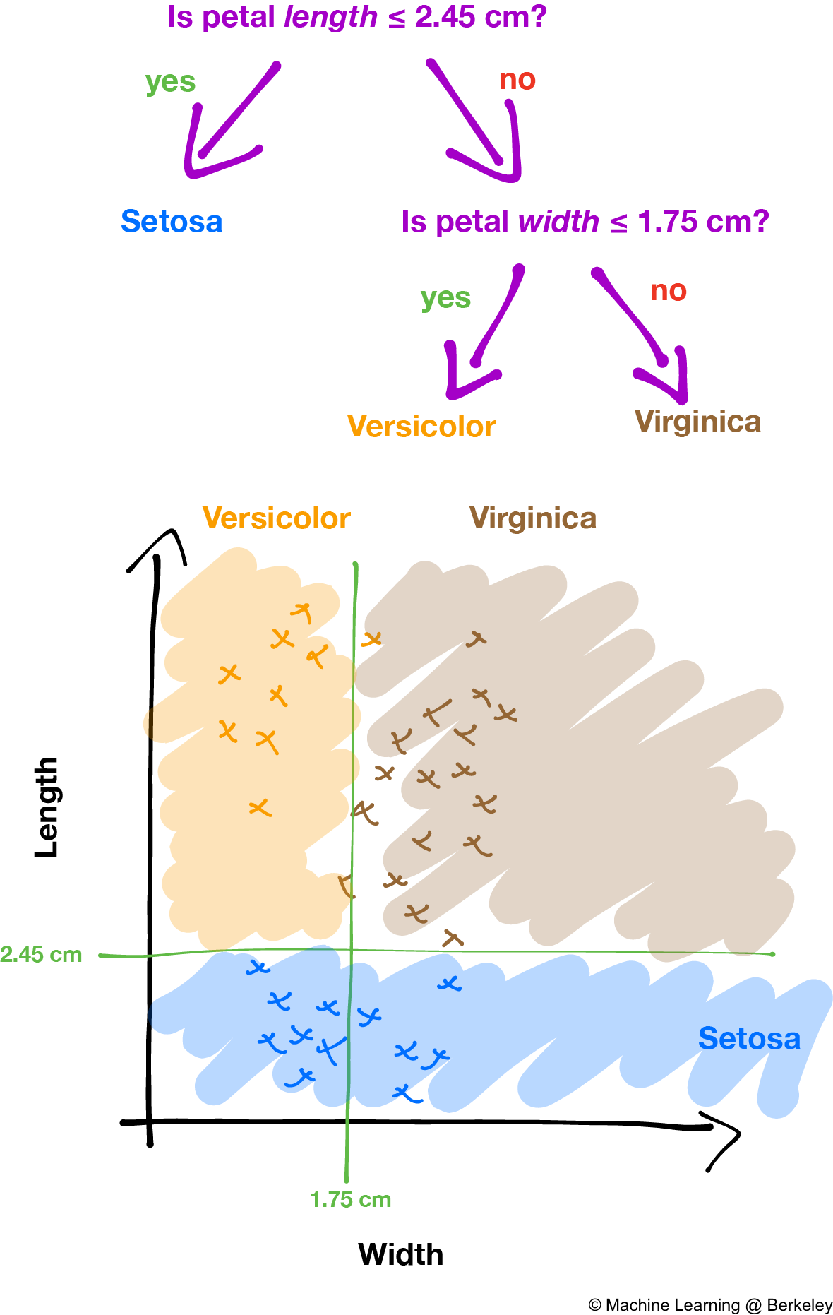
How a decision tree partitions the data into different classes. The decision boundaries create regions that can be associated with classes. Non-contiguous regions can also share the same class. Notice how the decision boundaries are always exactly horizontal or vertical; decision trees are great for creating "boxy" decision boundaries.
By varying the height (i.e. number of levels) of the decision tree, we can control the number of regions we split the data into. As always, trees that are too short can underfit, and trees that are too tall can overfit.
Regression
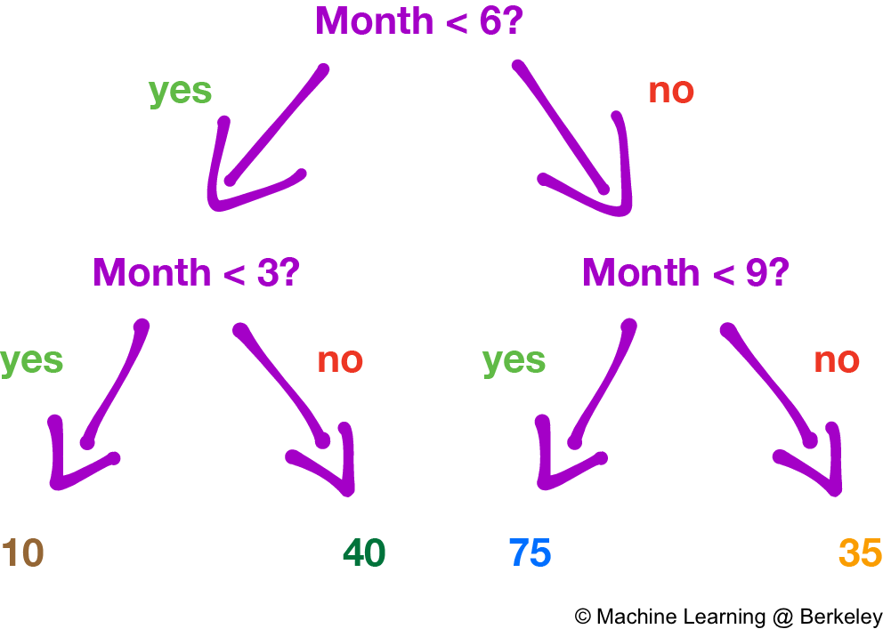
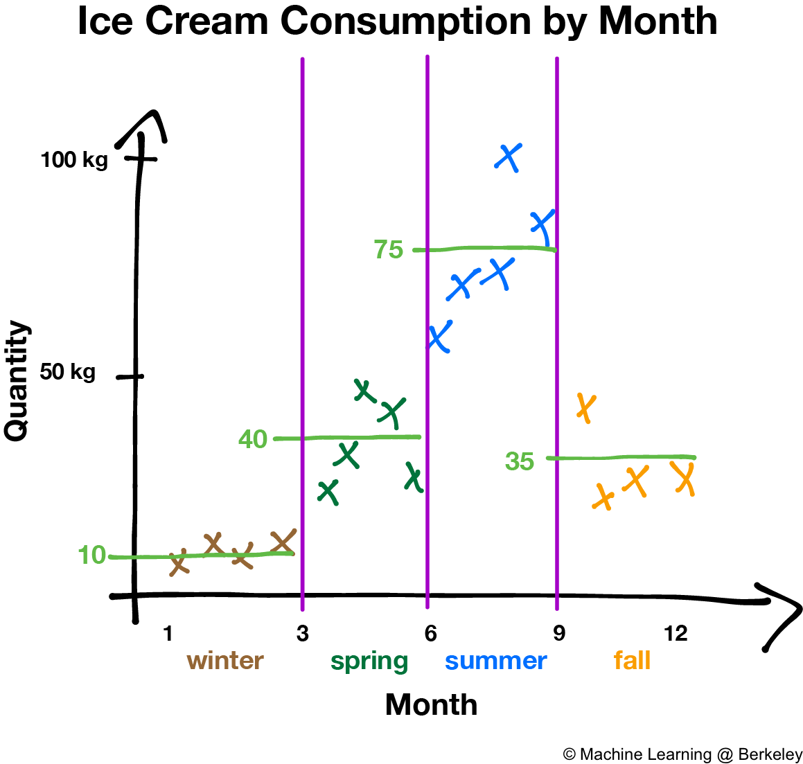
Regression and classification both function similarly for decision trees in that we choose values for the variables to partition up the data points. However, instead of assigning a class to a particular region like in classification, regression decision trees return the average of all the data points in that region. Why an average? Because it minimizes the error of the decision tree’s predictions.
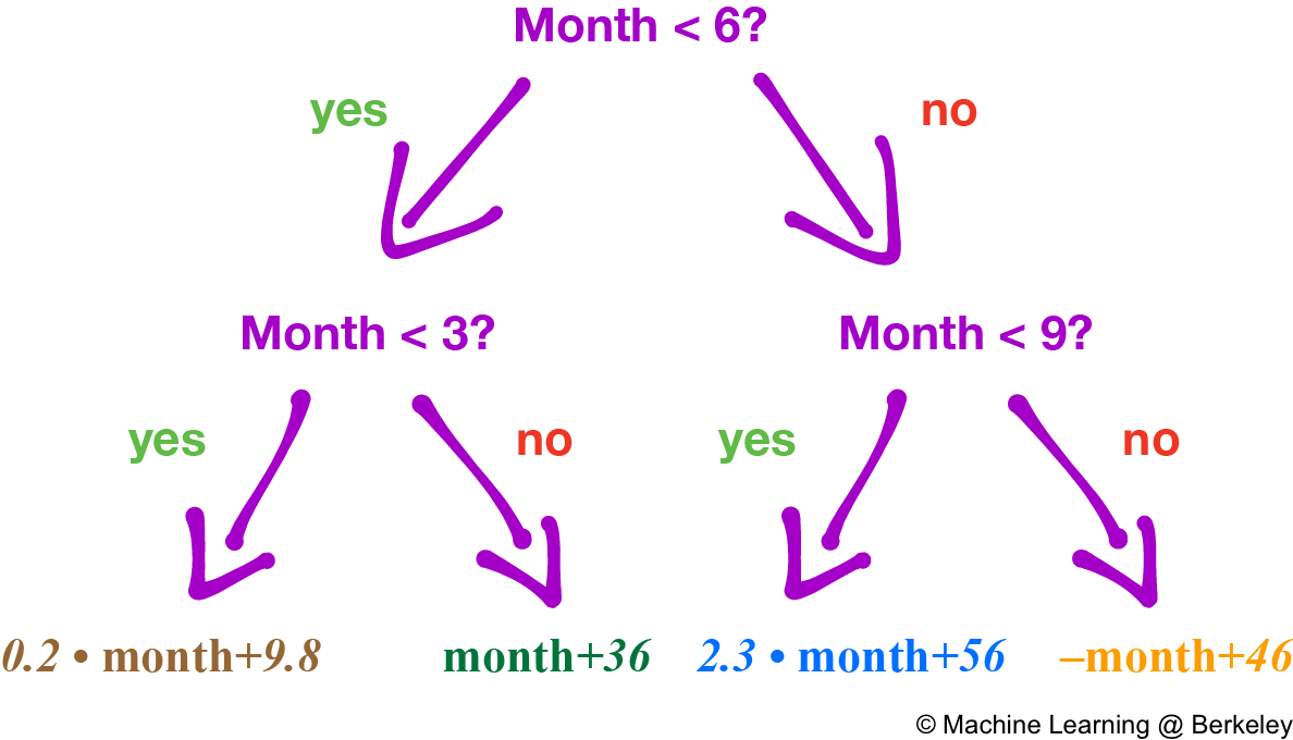
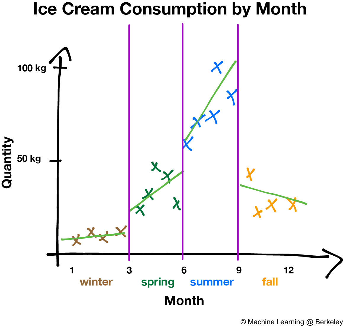
There’s also a variation where the decision tree fits a regression line to the data points of each region, creating a jagged piecewise line. However, trees constructed this way are more prone to overfitting, especially in regions with fewer data points, because noise is weighted more than it should be.
Training the Decision Tree
How do we tell if the variable and value that we’ve chosen is a good one? It helps to think of the decision tree as an “organizer”. If we were to organize a hundred blue and red socks into several drawers, would it be better if each drawer had a mix of socks of all colors or if each drawer only had socks of one color? Contrary to the wishes of lazy and disorganized children, drawers with socks of one color are more organized and easier to navigate.
Similarly, we’d like our decision tree to organize data points so that it separates data points (i.e., socks) into regions (i.e., drawers) that are as “pure” as possible. This means that as we are building the decision tree, we always choose the split that maximizes the amount of information we can conclude. More concretely, we choose a value such that each region is largely made up of data points from one category. By figuring out how “pure” each region is, we can figure out if our chosen value is a good one.
Imagine that a mother tells her kid to organize his sock drawer. Fifteen minutes later, he comes out and announces that he’s organized all the drawers by sock color. Like any good parent would, she goes and checks whether he made good on his claim.
She pulls open the drawer her good son kindly labeled “blue socks”. She reaches in and pull out a blue sock. Good. She is not surprised at all.
She pulls open another drawer labeled “red socks”. Reaching in, she pulls out a hairy spider as big as her hand! Like any normal parent would, she drops the disgusting thing and screams, leaving her son rolling around on the floor in laughter. We call this being infinitely surprised.
Let’s translate this situation into the language of math. We want to create a function \(f\) that converts what the parent expects (probability \(P\)) to how surprised she is when she observe a certain event (i.e., pulls something from the drawer): \(I(event)=f(P(event))\)
Based on the label of the “blue socks” drawer, the probability of finding a blue sock in that particular drawer is \(P(blue sock)=1\). Therefore when the parent does in fact find a blue sock in the drawer, she is not surprised at all: \(I(blue sock)=0\).
However, the probability of pulling out a spider from the “red socks” drawer is \(P(spider) = 0\); the parent was not expecting to see a spider at all. Therefore when she does pull one out, she is infinitely surprised: \(I(spider)=\infty\). She would similarly be infinitely surprised if she found a blue sock in the “red socks” drawer, albeit with less screaming.
To sum up what we’ve seen so far, \(P(event)=1 \rightarrow I(event)=0\) and \(P(event)=0 \rightarrow I(event)=\infty\)
How surprised is the parent overall? A simple way to figure this out is sum up the surprise that you’ve experienced so far: \(I(blue sock)+I(spider)\). In more general terms, if we observe two events \(A\) and \(B\), then our total surprise across both events is \(I(A\cap B)=I(A)+I(B)\). Plugging in our function from earlier, \(I(event)=f(P(event))\), we figure out that \(I(A\cap B)=f(P(A\cap B)\) and \(I(A)+I(B)=f(P(A))+f(P(B))\), which means that \(f(P(A\cap B))=f(P(A))+f(P(B))\)
We also know that observations at one sock drawer doesn’t affect observations at another sock drawer. That means each event is independent of each other, and we can multiply them together. So using probability theory, we determine that \(f(P(A\cap B))=f(P(A)P(B))=f(P(A))+f(P(B))\).
What functions give us this kind of behavior? Logarithms! But remember, we want \(P(event)=0 \rightarrow I(event)=\infty\), but \(\log(0)=-\infty\). Therefore our desired function \(f(P(event))=-log(P(event))=I(event)\), which now successfully determines how surprised we are.
Armed with this knowledge, we can look at a region defined by a leaf of the decision tree and calculate the expected surprise, or Shannon entropy as thus:
\[D=-\sum^k_{k=1}\hat{p}_{mk}\log{\hat{p}_{mk}}\]Where
\(K\) is the set of all classes or possible outputs of the decision tree
\(\hat{p}_{mk}\) is the probability (or proportion) of data points belonging to class \(k\) in leaf \(m\)
Now how does this relate to decision trees? Surprise in our analogy is actually related to the amount of information we gain from observing an event. Think about what makes us surprised; if we gain a lot of information from an event (a spider in a drawer), then we are a lot more surprised than when we observe what we expect to find (a blue sock in a blue sock drawer). Similarly, when we are given set of data, we have some initial amount of surprise for the set as a whole. We want to choose a split that decreases the amount of surprise in each region as much as possible. This translates to gaining the most information for the question we ask.
Ensemble Models
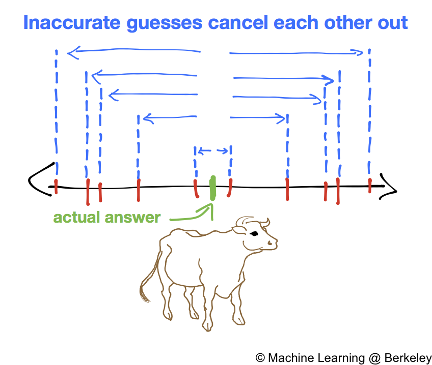
There’s a story of a fair where visitors would guess the weight of a bull, and whoever got the actual weight won a prize. The organizer noticed that although none of the individual guesses were exactly correct, the average of the guesses was surprisingly accurate. Why is this? Intuitively we can think of who’s doing the guessing. Some people are experts on certain things. A farmer is more likely to know the weight of the bull than someone visiting from a city, so he can make a reasonably accurate guess. City dwellers are more likely to be far off the mark (high variance). However, their lack of knowledge produces an interesting behavior: they are just as likely to overestimate the bull’s weight than underestimate. Thus the combined sum of their estimates yields a better estimate than any individual city dweller’s guess.
Although the cow story concerns regression, we can apply the same concept of aggregating a bunch of guesses to classification as well. If we have a bunch of classifiers, such as decision trees, we can aggregate them to create a much better classifier. Classifiers are simply models of any kind (decision trees, SVMs, neural networks, etc.) that can classify data better than random guessing. That means even though decision trees, like city dwellers, are individually not very accurate classifiers, combining their predictions yields a much more accurate result with lower variance, because it’s less likely for the majority of decision trees to guess incorrectly.
However, having multiple classifiers won’t be useful if they are all identical. So we must train them in ways so that they each specialize in some aspect of the problem. Two examples of this are bagging and boosting, which are covered in the next section.
Bagging and Boosting
Bagging (aka Bootstrap Aggregation):
In bagging, we throw our training data into a proverbial “bag” and repeatedly sample (take individual data points) from that bag, putting the data back into the bag every time. Then we use those data points to train our classifier. This is called sampling with replacement, or bootstrapping. By repeating this process with many classifiers, we can create multiple classifiers, all slightly different from one another.
Why put the data back into the bag again? Remember that we don’t want to train our classifiers on the exact same type of data. But if we don’t have a lot of data, the amount of data we can use to train each classifier becomes quite limited. Replacing the data point every time we sample allows us to maintain the distribution of our data, and reduces the amount that our final classifiers’ predictions vary from input to input due to the fact that each training subset is statistically representative of the full dataset.
When actually using the ensemble to classify data, we have every classifier make a decision. The ultimate decision of the ensemble is decided by majority vote among the classifiers (in the case of classification) or by an average of all the classifiers’ individual predictions (in the case of regression).
Why does bagging reduce variance of the final ensemble model’s predictions? From basic probability theory, we can represent the decision trees as a set of i.i.d (independent and identically distributed) predictions from \(N\) different decision tree models (\(Z_1, Z_2, Z_3,... Z_N\)), which each have variance \(\sigma^{2}\). These N different decision tree models are trained on N different samples of the original data generated via a statistical technique called Bootstrapping, where we sample observations with replacement from the original datasets to create several different datasets.
But if we combine the \(N\) predictions into one prediction by averaging them, the variance of the combined prediction will be \(\sigma^{\frac{2}{N}}\). Hence, averaging out the predictions of multiple classifiers will drastically reduce the variance of our bagging ensemble classifier which combines these \(N\) different decision tree models, assuming that they are all different decision tree models, independent, and trained on slightly different datasets.
Random Forests
We can train many decision trees and use them as classifiers, creating a random forest. However, there remains a major problem with bagging decision trees: What happens if the individual decision trees are too similar? In other words, what if they all ask the same questions? Then we lose the benefit of having multiple decision trees, because they will all behave exactly the same; if one decision tree misclassifies something, chances are that the other decision trees will also make the same mistake. Can we modify our original approach to bagging so that we can create even more diverse sets of decision trees?
Let us describe the random forests approach more formally. Let’s say we are trying to predict home prices with 9 variables, such as size, location, square footage, proximity to schools, neighborhood characteristics, and the number of bedrooms. We can take our original data and generate several samples from the original dataset using bootstrapping. We now train N decision trees on each of the N different samples (same as before), but with one major caveat. In the process of training these decision trees, whenever we make a new split in a tree, we select amongst a randomly chosen subset (of size \(m\)) of the \(p\) variables as possible candidate variables to split upon. At each new split point, we randomly choose \(m<p\) variables to be in our subset of candidates, and consider only those m variables. So, for our first decision tree’s first split point, let’s only consider location, square footage, and number of bedrooms (\(m = 3\)) while ignoring the remaining 6 features (\(p = 9\)). Typically, \(m\) is chosen on the magnitude of the square root of p in order for the random forests procedure to produce reasonably decorrelated decision trees. Once we have N different decision tree models, we can average all of their predictions like we did for bagging to get our ensemble model’s final prediction.
Boosting
Adaboost
Imagine a bunch of people are sitting around a table making an important business decision for their company, such as deciding how much to buy a startup for. Everyone wants the company to do something slightly different, so how do you, the leader, ultimately decide what to do? One option is to evaluate use past experiences to decide how much you want to trust each person’s decisions. If someone historically has made bad decisions, it would make sense to trust them less than someone who has never led the company astray. For example, an unreliable person suggests to buy the startup for 20 million but an experienced veteran values it at 50 million, and you privately think it’s worth around 30 million. You most likely trust yourself, and you trust the veteran more than the unreliable person, so it makes sense to ultimately set the valuation of the company somewhere between your personal valuation (30 million) and the veteran’s valuation (50 million).
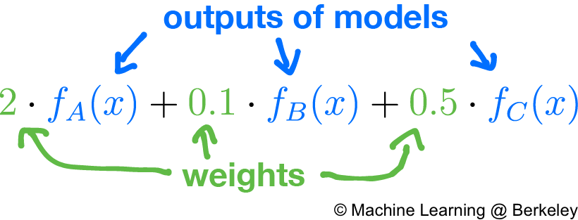
Adaboost, a well-used boosting algorithm, functions on a similar principle. Given a bunch of regression or classification models, it judges the credibility of each model by testing it on a test set. If a particular model has high accuracy, we will trust it more. Conversely, if a particular model has low accuracy, we will trust it less. In this case, by “trust” we mean how much influence, or weight, the model’s decision has over the overall result. So instead of taking a simple average of all the models’ outputs, we take the weighted sum of their output, where the weights are directly proportional to the accuracy of each model. In fact, you can think of the average as a simple weighted sum where all models are weighted equally.
In the case of regression, the output of the ensemble model will be the raw weighted sum. However, in the case of classification, the output will be based heavily on what the output should be. For example, if the output is “yes” or “no”, then we could arbitrarily make values > 0.5 mean “yes” and values ≤ 0.5 mean “no”. If there are more classes, we could switch to using vectors to represent the different choices, such as <1, 0, 0> to mean class 0, <0, 1, 0> to mean 1, and <0, 0, 1> to mean 2. Then by taking the weighted sum of all the outputs we get a vector such as <0.24, 0.8, 0.7>. Since 0.8 is the largest number, and it’s position indicates its class is 1, then the overall output of the ensemble model is class 1. This is called one-hot encoding.
Regression
We can also use another method for boosting regression models. Let’s use the previous scenario of predicting the price of a house.
First, we train a decision tree on all the inputs in the training data, which can be treated as a function \(f_1(x)\). This decision tree is bound to have predictions that are slightly off from the actual values, so we figure out the error for each prediction. For example, if our decision tree guessed 100k for the price of a house when the actual price was 75k, then our error is
\(\text{error} = \text{actual value} - \text{predicted value} = 75k-100\text{k} = -25\text{k}\).
This tells us that if we had subtracted 25k (or equivalently added -25k), then we would have obtained the correct solution. More generally,
\[\text{actual value} = \text{predicted value} + \text{error}\]How do we improve our prediction? One way is to create a second decision tree \(f_2(x)\) that predicts the error of the first tree. Because as observed earlier, if we can add the error to the predicted value of the first tree, we will obtain the actual value!
In other words, \(y\approx f_1(x)+f_2(x)\)
Nevertheless, our second tree will still have errors in its prediction. As a result, we train a third decision tree to predict the errors of the second, and so on until we have trained some prespecified number of decision trees. Then, we simply add the predictions of all the decision trees to obtain a more accurate result.
However, putting so much effort into correcting errors tends to leave the ensemble, or forest, of decision trees prone to overfitting, because as you build more and more decision trees to correct errors made by the previous decision trees, even small errors and noise in the data will be “predicted” and corrected, resulting in an ensemble that is very accurate on training data, but not as accurate on testing data.
Bagging vs. Boosting
Before we try applying novel forms of ensemble learning to decision tree, let’s understand the basic strategies that both bagging and boosting utilize to create a diverse set of classifiers. In bagging, we create multiple copies of the original training data set using bootstrapping, fit several decision trees to each of the different copies, and take the average of all the predictions of all the trees to make our final, overall prediction in the final ensemble model. On the other hand, in boosting, we iteratively train a decision tree on the error of previous decision trees, slowly generating our final ensemble model which is a linear combination and summation of our individual decision tree models.
Conclusion
Before neural networks became popular, decision trees were the state of the art for Machine Learning. Although current models based on neural networks often outperform decision trees and random forests, there is much to gain by utilizing the techniques for ensemble models outlined in this post. With ensemble models, you can leverage the power of multiple models, including decision trees and neural networks, to compensate for the individual irregularities or weaknesses of each model.